Changes to mean-reversion rate model
Low gas prices: is the mean-reversion gone?
In the first week of September this year, the TTF gas spot prices went below 7.50 €/MWh. This was almost four times as low as 12 months before, when prices were over 28 €/MWh. Together with the other European natural gas prices, it had been in almost continuous decline ever since. We slightly adjusted our mean-reversion rate model to better reflect these prices swings on the gas market.
There were two main factors for this trend. After an exceptionally mild winter, gas storages were well stocked in 2019, and relatively low volumes of gas had to be injected over the summer to be full again for the next winter. When that coincided with abundant global gas supply this summer, leading to a large influx of LNG into Europe, the prices were consistently pushed down.
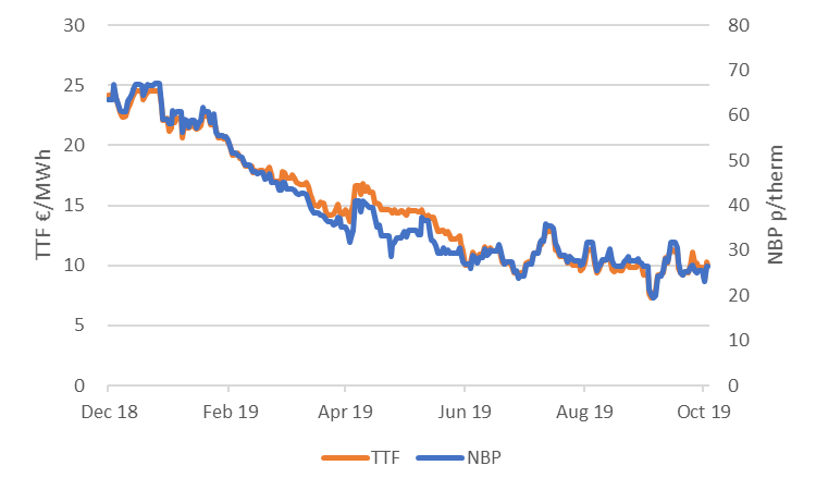
Figure 1: Northwest-European gas spot price development
Mean-reversion rate
Unfortunately for gas storage traders, there was limited benefit of the low prices, because storages were almost full already. The level of volatility was good though: amidst the downward trend were various short-lived periods of up- and down moves. When these cycles can somewhat be predicted, then an active spot trading strategy can generate money. In financial modeling of gas storages, this predictability of the price cycles is captured by the mean-reversion rate. More exactly, the ‘standard’ time-series equation for gas spot prices takes the following form:
![]() Where InS(t) is the natural logarithm (ln) of the spot price S(t) on day t, α is the daily rate of mean-reversion, μ(t) is the mean-level to which the ln of the spot price reverts, ε(t) is the random part of the daily spot price return (standard-Normal) and σ its standard deviation.
Where InS(t) is the natural logarithm (ln) of the spot price S(t) on day t, α is the daily rate of mean-reversion, μ(t) is the mean-level to which the ln of the spot price reverts, ε(t) is the random part of the daily spot price return (standard-Normal) and σ its standard deviation.
In a 1-factor model, the mean-level μ(t) is constant or follows a pre-defined seasonal pattern; the random spot returns ε(t) are the only random element of the spot prices. In a multi-factor model, as is embedded e.g. in the KyStore storage model, the mean-level is a random process itself. It captures the fact that spot prices respond to movements in the forward market: when forward prices go up, spot prices tend to go up as well, and vice versa.
When estimating the parameters of this mean-reverting process, it is generally assumed that the mean-level equals the ln of the front-month (M+1) forward price. The idea is that the front-month is a very liquid product that is most nearby to the spot, so a natural point to which the spot price will move. Temporarily, e.g. due to a spell of cold weather, it could move away from this mean level, but eventually it has to move back. In line with the time-series model, the next graph shows the difference between the ln of the spot price and of the front-month forward price for the TTF market. For example, when this difference is +10% it basically means that the spot price is 10% above the front-month price.
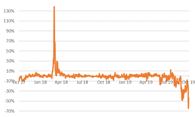
Figure 2: Difference between TTF spot and front-month forward price, both measured in natural logarithm.
Spot price movements
Most of the time, the line in the graph hovers around 0, which is in line with the concept of mean-reversion. There are two main exceptions though. During the cold spell in February-March 2018, spot prices spiked, while front-month prices moved far less. In fact, the spot price volatility was extremely high, and spot prices reverted to the front-month with some delay.
The other exception started to develop around August this year: spot prices were consistently below front-month prices. This pattern reflected the expectation of traders that spot prices next month would be 10 to 50% higher than in the current spot market. In such market conditions, the mean-reverting model seems to be flawed.
However, relatively simple enhancements are possible. The front-month price is just a proxy for the mean-level, which itself is actually unobserved. It can be better approximated when we adjust for the seasonality in the forward curve. For example, spot prices in March are higher on average than in April, so spot prices in March will be mean-reverting to a slightly higher price than the April forward price. This seasonal spread can be estimated from the difference between March and April forward prices at the time that both were traded. For example, we can take the last 5 trading days in February and compute the spread in the ln of the March and of the April forward price. Let’s denote the result C(m) for each month m and add this to the equation together with the front-month price F(t), so we get:
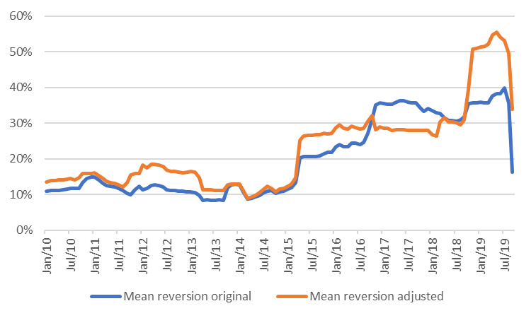
Figure 3: Mean-reversion rate estimated with the adjusted mean-reverting model.
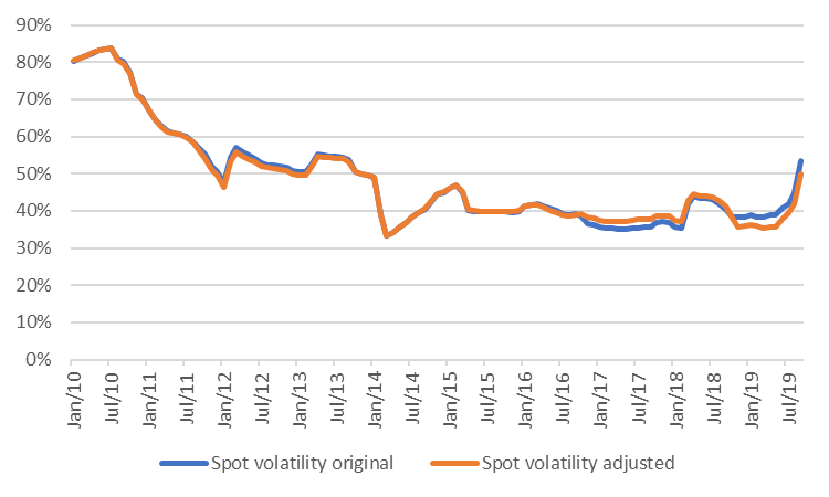
Figure 4: Spot volatility estimated with the adjusted mean-reverting model.
Conclusion
Figure 3 and 4 show the estimated parameters for the TTF market using a 2-year moving window, with the original and the adjusted specification. Except for 2017, the adjusted model has a higher mean-reversion rate and a slightly lower (residual) spot volatility. Especially in the last 12 months the adjusted model performs better.
Nevertheless, the large variations in both mean-reversion rate and spot volatility also highlight that no model is perfect. This type of model assumes that the price dynamics follow a stable pattern with fixed parameters, whereas prices tend to behave differently in some periods than in others. This is a general challenge with time-series modeling, but maybe even more so in energy markets, where profound structural changes take place from time to time.
To view this article as a pdf: White paper low gas prices 2019
Author: Dr Cyriel de Jong
Date: 3 October 2019