PPA Insights: Fundamental modelling of power markets
PPA Insights: The financials of renewable power and PPA Contracts
Author: Cyriel de Jong, KYOS Energy Analytics
Introduction to fundamental modelling
How can we generate realistic forecasts of future power prices? Here is where fundamental power market modelling makes its appereance. In the previous article, we have seen that the merit order provides a useful starting point, but lacks sufficient detail for any serious investment analysis or PPA valuation. In this article we explain fundamental power market modelling, which takes us to the required level of detail. It allows us to take into account start costs, energy storage and many more important features of real-life power markets.
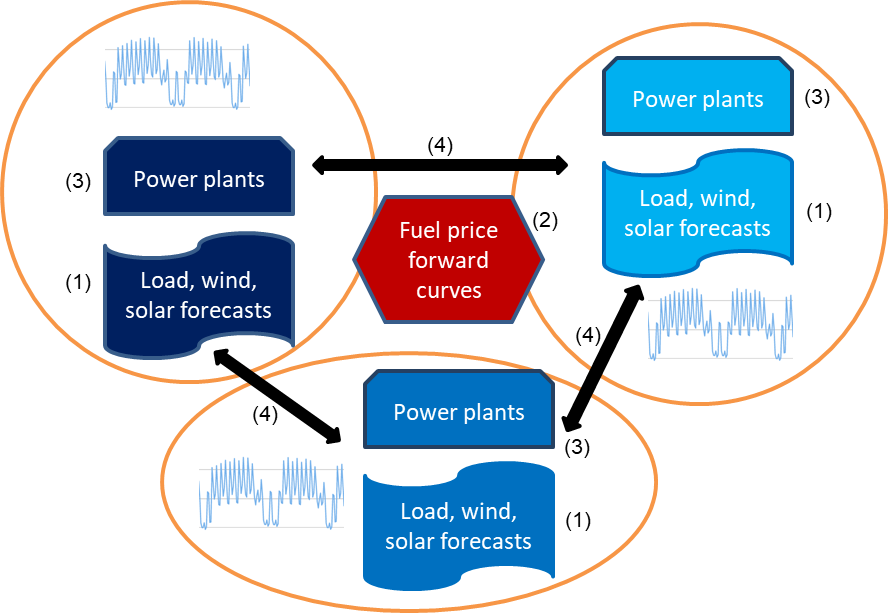
Figure 1: Schematic picture of a fundamental power market model with inputs of three markets. The different elements (1)-(4) are described in the main text. Source: KYOS.
Figure 1 shows the main inputs to a fundamental analysis of multiple power markets. Each orange circle or ellipse represents a power market area. The forecast of the power demand, minus the forecast of non-flexible generation from solar, wind and hydro, is the so-called residual load (1). Fuel and CO2 price forward curves (2) and detailed information about power generation assets (3) determine the variable production costs of all flexible generation assets. Note that batteries and other forms of energy storage should also be included in the power plant list. Finally, interconnection capacities (4) allow power to flow from low-priced areas to high-priced areas until prices are equal in both areas or until the capacity is fully utilized. Of course, there are several more inputs, but these are the main building blocks. In the remainder of this article, we will zoom in on the different elements.
Beyond the merit order
The merit order contains the variable costs of the various power generation sources, sorted from low to high. A fuel-fired power plant has different cost components, and it is not straightforward to express the variable costs in a single number. First of all, there are fixed costs, in particular resulting from the original investment (financing costs), but also certain fixed costs to operate the plant and pay the personnel. Fixed costs can be considered ‘sunk’, meaning that they do not change with the power output.
Secondly, there are variable costs, which move with the power output. The fuel and emission costs are generally the main variable costs, followed by start costs and the variable part of the operations and maintenance costs. Once a power plant has been constructed, only the variable costs determine the optimal dispatch. The optimal dispatch is considerably more complex than the merit order seems to suggest. We take a combined-cycle gas turbine as an example to demonstrate some of the complexity.
Suppose that the higher heating value (HHV) efficiency of the combined-cycle gas turbine (CCGT) is 50%, which means that 2 MWh of natural gas need to be bought in the market for each MWh of power. Natural gas has a carbon (CO2) content of 0.205 ton per MWh. This means that if the gas price is 15 €/MWh and the carbon emission price 20 €/ton (the cost of emission allowances in the EU ETS), the fuel and emission costs per MWh are:
- Fuel cost = Gas price / Efficiency = 15 / 50% = 30 €/MWh
- Carbon cost = Carbon price * Carbon content / Efficiency = 20 * 0.205 / 50% = 8.20 €/MWh
Ignoring any other variable costs, the market price should be at least 38.20 €/MWh for this plant to produce. Or stated differently, if the power price is 45 €/MWh, the gross margin or clean spark spread is 6.80 €/MWh.
Bidding in at variable or marginal costs?
In reality, whether the plant produces, and at what exact output level, depends on more factors than the fuel and emission costs. One element is that the overall efficiency is not constant, but is lower when the plant produces less than its maximum. For example, a gas-fired plant may produce in a range between 180 and 400 MW, with HHV efficiencies rising from 44% to 50%. A higher efficiency results in a lower average cost. Although the average efficiency increases, the marginal efficiency decreases: for each extra MWh of power, progressively more fuel is needed (Figure 2).
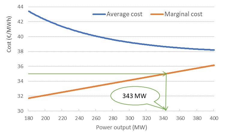
Figure 2: Average and marginal costs of production for a gas-fired power plant described in the main text. The green arrow points where the marginal costs of production equal the market power price of 35 €/MWh. It shows that 343 MW is the optimal output level. Source: KYOS.
Now suppose the power price is 35 €/MWh, let’s consider two possible situations:
- The power plant has no start costs and can turn on or off in each individual hour. This is realistic for a very flexible gas engine. A market price of €35 is not sufficient to recoup the variable costs of 38.20 €/MWh, so the plant will not produce.
- The power plant has to produce in this hour, for example because it cannot turn off for a single hour, or turning off (and later on) is too costly due to start costs. Now the marginal costs are decisive for the optimal dispatch. When the plant produces 343 MW, its marginal costs are equal to the market price of 35, and hence 343 MW is the optimal dispatch.
Start costs and more
The merit order of a market is a useful albeit simplified picture based on the average variable costs. It can serve as a starting point to assess the potential level of future power prices, but does not reveal everything. Elements that should be considered for fuel-fired plants include:
- The minimum and maximum output levels and efficiencies, as explained in the example
- Start costs, start times and ramp rates
- Minimum on-times and minimum off-times.
- Impact of ambient temperature on efficiencies and output levels.
- Maintenance and unexpected plant trips.
- Must-run obligations, e.g. to generate heat or steam.
In the second situation, the CCGT will only produce if there are hours before or after with a price well above 38.20 €/MWh. Otherwise the start costs will not be recovered and the plant is producing at a loss. For example, if the start costs are €12,000, then the total spark spread of a production sequence must at least be €12,000. Spread out over 12 production hours of 400 MW, the minimum spark spread is 2.50 €/MWh to recover the start costs.
The other factors mentioned above are highly dependent on the individual CCGT, but do need to be taken into account in the bidding price. The example shows that it is not easy to derive the prices at which plants bid into the market, even if the market is fully competitive and there is no strategic behavior.
Hydro power and energy storage
The power supply consists of at least three other types of generation: hydro power, energy storage, solar and wind power. Their behavior is very different from fuel-fired generation and is not easily captured in the merit order.
Bidding energy storage into the market is actually quite complex, because it is not the absolute price level that matters, but the relative differences between the hours. With the expansion of renewable (intermittent) power generation, energy storage is becoming increasingly important to balance the system. It is therefore essential to incorporate it in a realistic way in the fundamental model, allowing for a variety of asset parameters, such as:
- Total energy storage capacity (MWh)
- Rate of storage (MWh/h)
- Rate of production (MWh/h)
- Efficiency or energy loss during a full cycle (%)
- Variable costs of operation
Just like the conventional generation assets, the energy storage assets should be optimally dispatched against market prices.
Solar and wind
A fundamental model treats solar and wind power production, together with demand, primarily as non-flexible (intermittent) elements in the power system. They are exogenous inputs to the system optimization. Forecasts of demand and intermittent renewable generation are often derived from economic and policy scenarios, such as published by the IEA, European Commission, EIA, or national governments. Such scenarios generally stipulate future capacities for renewables and a certain percentage change in electricity demand. The challenge is to translate those macro-economic numbers into detailed hourly forecasts.
A common approach is to take a specific historical base year, e.g. 2018, for which the actual hourly demand and renewable production are known. These numbers are then scaled up or down to reflect the forecast growth rates in demand and production. Various refinements are possible, for example to take into account changes in electricity demand profiles or renewable production load factors. The advantage of taking a specific base year is that it incorporates real-life fluctuations, e.g. due to weather variations. A disadvantage is that the forecast becomes very dependent on what happened in that particular base year. If the base year had a very sunny month of May, then all forecast years will have a very sunny May, with a lot of solar output. To alleviate this problem, it is therefore recommended to run the same analysis with multiple base-years, and average the outcomes across the runs to obtain a single forecast.
Optimization in a fundamental power market modelling
Together with the expected future demand and (non-flexible) hydro power production, the expected future solar and wind production are essential ingredients in a power price forecast. Basically, a detailed fundamental model works as follows:
- Forecast residual demand = demand – solar/wind/hydro production
- Forecast the fuel and emission prices (via the forward curve or with simulations)
- Find the power price in each hour, such that:
- The output of all flexible generation and storage ≥ residual demand
- All the flexible generation and storage is optimally dispatched against the power prices, taking into account all production costs and (non-)flexibilities; i.e. we find the prices which allow demand to be met in each hour at lowest system cost.
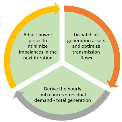
Figure 3: One iteration in the main part of the optimization algorithm using Dynamic Programming (DP) and Lagrangian multipliers in a fundamental power market model.
In case of interconnection capacities to other markets, a distinction must be made between the core- and non-core markets. The core-markets are jointly modelled in detail. The use of their interconnection capacities is part of the optimization in step 3. In principle, when the power price in market A is below that in market B, export from A to B must happen until both prices are equal or until the maximum interconnection capacity is utilized. The non-core markets are modelled simpler or not at all. In the latter case, in step 1 the forecast net export from core- to non-core markets is added to the demand forecast of the core market.
The optimization in step 3 described above can be fairly complex and time-consuming. Many fundamental models are based on some form of Mixed Integer Linear Programming (MILP). This is a very generic way of formulating the optimization problem, which can then be solved by commercial solvers, such as IBM-CPLEX or Gurobi. A different solution approach is incorporated in the KYOS fundamental model KyPF. It uses dynamic programming and Lagrangian multipliers, following the seminal work by Richard Bellman (1956).
The KyPF model performs different iterations, in which alternately the flexible generation is optimally dispatched (using dynamic programming) and then the hourly power prices (the Lagrangian multipliers) are adjusted depending on the level of imbalance. For example, if the total generation in some hour and iteration is 30,000 MWh, while the residual demand is 32,000 MWh, the price in that hour is lifted with the aim to minimize the imbalance in the next iteration. Adjusting the power prices is simultaneously done for all hours and all markets before a new iteration begins. Typically, around 15 such iterations suffice to reduce imbalances to less than 1% of the residual demand. Over a horizon of around 10 years, and with 14 European ‘core’ countries with a total of 1,600 flexible power generation assets, the calculation takes around 1.5 hours in the online KYOS Analytical Platform.
These balancing iterations also implicitly capture the costs of balancing the power market in the forecast, which in reality happens on an hour-to-hour basis dependent on the supply and demand imbalance. As mentioned in the previous article, the value of renewable PPAs is affected negatively by these balancing costs due to the intermittent nature of power production from solar and wind farms.
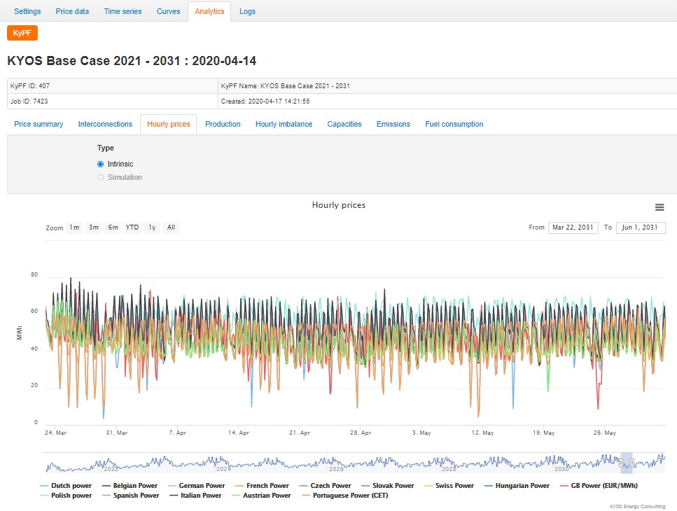
Figure 4: The hourly power price forecast of the KyPF model for 14 European countries. The calculation has been performed over an 11-year horizon (2021-2031), but the graph narrowed down to around 2 months. Source: KYOS Analytical Platform.
Ingredients of fundamental modelling
In a detailed fundamental market model, all elements in a power market are included with sufficient detail and with hourly granularity. Leaving out an essential element, can have a big impact on assumed profitability of a future investment or PPA contract. One such crucial element is the start costs of fuel-fired power plants.
Figure 5 shows the impact of those costs on the German power prices. The results have been generated with KyPF, the KYOS fundamental power market model. On average, the inclusion of start costs raises the average power prices in 2021 by only 1 €/MWh. Considerably more significant is the impact on the hourly dynamics: with start costs the difference between high- and low price hours becomes larger. In the hours with high (residual) demand, the price must be high enough for flexible plants to start up. In hours with low demand, some plants prefer not to turn off but rather run on minimum load; that leads to a soft form of must-run, which pushes the prices down in low-demand hours. The net effect is that price changes between hours are about twice as large due to start costs of fuel-fired power plants.
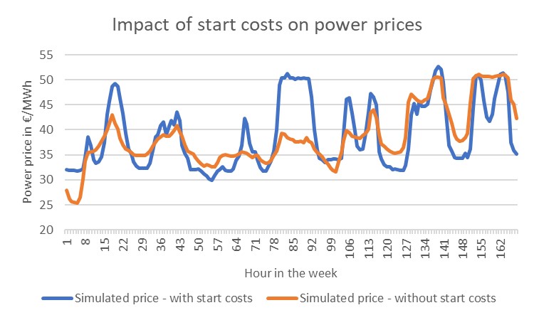
Figure 5: Hourly power prices for the German power market, generated with the KYOS fundamental power market model KyPF. The graph shows the second week of 2021. The inclusion of start costs for fuel-fired plants (blue line) leads to considerably more variation in prices. Source: KYOS Analytical Platform.
A wealth of information
In this article we have explained the principles of fundamental power market modelling. A detailed fundamental model uses relatively detailed inputs of all relevant assets. The non-dispatchable renewable generation (solar, wind, geothermal and part of hydro) enters the model in the form of hourly forecasts over the full evaluation horizon. The fundamental modeler also provides forecasts of fuel and emission prices, forecasts of electricity consumption, and forecasts of interconnection capacities. This requires a lot of data gathering, but is also very rewarding: the end result is not only an hourly power price forecast, but a detailed understanding of how the market could evolve, and plenty of opportunities for sensitivity analysis. In the next article we present a number of practical examples of how this information can be used to assess the financials of renewable power and PPA contracts.
To read this article in pdf: Fundamental modelling of power markets – the financials of renewable power and PPA contracts
Feedback on our “Financials of renewable power and PPAs”
We have written the articles to share our knowledge and hope it provided a useful source of information for newcomers and experienced professionals alike. Whether you are buying electricity for your company, developing new projects, working for a utility, providing financing, drafting policies, or just generally interested: we hope you have read the articles with interest and share your feedback with us: info@kyos.com.