PPA Insights: Production patterns of wind and solar
Author: Cyriel de Jong, KYOS Energy Analytics
Production patterns of wind and solar
The financials of renewable power and PPA contracts
In this article we take a detailed look at the production patterns of electricity generation from wind turbines and solar PV (solar photovoltaics). What are the main parameters determining the production? What is a power function, a load factor and the wake effect?
Setting the scene
As examples throughout the series of articles, we take an off-shore wind turbine in the North Sea and a solar farm in central Spain. The first parameter determining the production is the rated (or maximum) capacity. In this case, we assume this is 8 MW. Comparing capacities can however be misleading: an important parameter is the load factor or capacity factor. This is a percentage indicating how much the asset generates ‘on average’ over a year. It could e.g. be 50% for the off-shore wind turbine and 18% for the solar farm. A load factor of 50% for an 8 MW turbine leads to an expected annual production of 365.25 x 24 x 8 x 0.50 = 35,064 MWh.
Impact of load factor on production patterns
A high load factor is important for investors, because it increases the revenues per MW of capacity. It also implies a more stable production, and hence a more efficient use of the network cables. In combination with good predictability of the fluctuations, a high load factor of renewable generation requires fewer flexible assets in the system (energy storage, gas-fired plants, hydrogen). A high average production is likely to become more and more important in the future, and explains why off-shore solar farms with load factors of around 15-20% have higher network costs than off-shore wind farms with load factors of 45-55%. Even higher load factors and more stable production can be achieved with ocean energy (tidal or waves), making it an interesting addition to the energy mix.
The load factor is an easy number to communicate, but is actually a result of the local weather conditions and the power curve of the asset. The power curve describes how the (main) weather variable, such as wind speed or solar radiation, is transformed in electrical power. As an example power curve for the wind farm we take data from the Vestas V164-8.0 [1] (see figure 1).
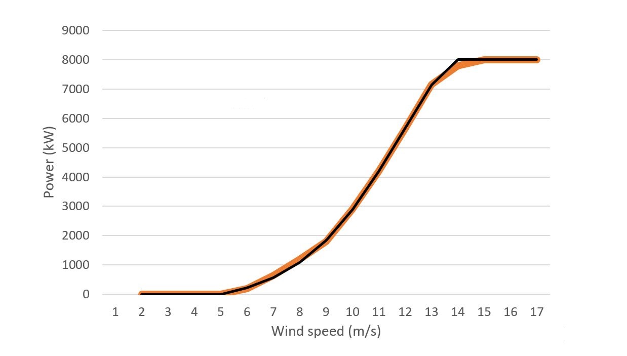
Figure 1: Power curve for the Vestas V164-8.0: power generation for different wind speeds. The black line shows the Sigmoid function which closely matches the actual (published) data points.
Power curve wind
The S-shape of the wind power curve is very typical. It is often described as a Sigmoid function, for example with the following parameterization where W is the wind speed, V(W) the corresponding power output, and a,b,c,d the parameter values, all larger than or equal to 0:
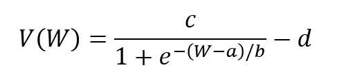
The function has a few nice interpretations which help to understand the role of the parameters. Firstly, when the wind speed is very (even infinitely) high, the output equals c – d. Secondly, the Sigmoid function has maximum steepness when the windspeed W equals a. At that point the output equals c/2 – d. This point is often reached around halfway between 0 and the maximum capacity. In that case, we can set d equal to 0 and c equal to the maximum capacity. The parameter b mainly determines the steepness by which the power generation increases with wind speed: a lower b results in a steeper slope.
For a closer fit with the actual output, the function can be constrained in the range between 0 and the maximum capacity. We could additionally specify a cut-in wind speed to keep production at zero for wind speeds below this level, in this case 3.5 m/s. With a relatively simple solver, such as the one included in Excel, one can obtain the best fitting parameters of the power function. When we add these additional elements (min, max, cut-in), the power curve of the Vestas turbine closely follows a Sigmoid function with parameters a = 9.97, b = 1.99, c = 11.97, d = 0.35.
Impeding factors on wind: blockage and wake
Note that other parameters than wind speed or solar radiation, such as temperature and humidity also play a role in reality; the power curves are valid for ‘average’ weather conditions. For wind farms at least two other factors play a role, the blockage effect and the wake effect. The blockage effect arises from the wind slowing down when approaching the wind turbines.
The wake effect impacts the effective wind speed of turbines within a wind farm and neighboring wind farms. Wind leaving the turbine will have a lower energy content than the wind in front of the turbine. This wake leads to reduced, and more turbulent, effective wind speeds behind the turbine. As the wind flow continues, the wake spreads and the wind speed recovers. This is especially important in larger wind farms: when more area is being used, the wake effect becomes more significant.
Solar electricity production patterns
For solar PV panels, the relationship between solar radiation and electricity production is simpler, and follows a linear pattern. Temperature also plays a role, with higher efficiencies at lower temperatures: a well-cooled floating solar park therefore produces more than rooftop panels. For our example, the power production per square meter of solar panel can be described as a function of solar radiation R and ambient temperature T as:
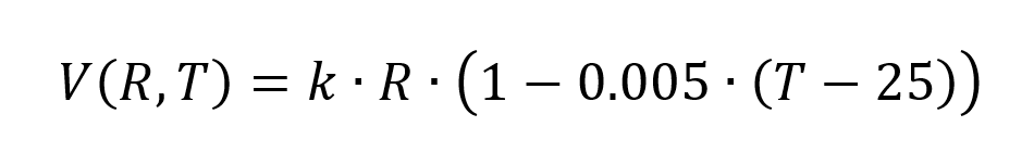
In this equation the parameter k is the efficiency of transforming the energy from the sun into electrical power and could be 16%. With solar radiation (R) of 1,000 W per square meter and 25 degrees Celsius ambient temperature (T), a 50,000 m2 solar park produces 8 MWh of electricity per hour. The last part of the equation takes into account the increase in efficiency with lower temperatures, in this case from 16 to 17% when temperatures drop from 25 to 5 degrees Celsius.
Adjustments for non-productivity
For all types of renewable generation, we have to make some adjustment for maintenance and outages. Whereas solar panels require very limited maintenance and will rarely have outages, wind turbines are more often out of operation, in between 1-5% of the total operational time.
Finally, renewable assets may be unavailable due to forced or voluntary curtailment. Curtailment may be due to local network bottlenecks or due to a general overproduction in the system. As mentioned before, to avoid such situations from happening, a stable production level and hence a high load factor are key aspects. It can also minimize the impact from voluntary curtailment, i.e. suspending production due to negative spot power prices.
Next article will be on Meteorology
In the upcoming two articles, the weather itself is the main subject. How can we gather data of wind speeds, solar radiation and ambient temperature? What are the seasonal and intra-daily patterns? And how does this transform into scenarios and forecasts of future production? To what extent are those production scenarios correlated between different locations or markets, and between solar and wind? There is enough to discuss in the next articles.
To download this article as pdf: Production patterns of wind and solar – the financials of renewable power and PPA contracts
Feedback on our “Financials of renewable Power and PPAs”
We write the articles to share our knowledge and hope it provides a useful source of information for newcomers and experienced professionals alike. Each article will be a mix of qualitative description, some mathematical formulations and numerical examples. Whether you are buying electricity for your company, developing new projects, working for a utility, providing financing, drafting policies, or just generally interested: we hope you read the articles with interest and share your feedback with us: info@kyos.com.
[1] https://en.wind-turbine-models.com/turbines/318-vestas-v164-8.0#powercurve