PPA Insights: Valuing long-term investments and PPA contracts
The financials of renewable power and PPA contracts
Author: Cyriel de Jong, KYOS Energy Analytics
Valuing long-term investments and PPA contracts
 Renewable energy investments have an economic lifetime of at least 15 years and hence investors seek for long-term PPA contracts to provide financial security. Both PPA buyer and seller have to form an opinion about the longer-term level of power prices.
It is impossible to forecast the future power price over such horizons with high accuracy, but it is possible to form your own view with a fundamental power market model. A fundamental power market analysis yields a wealth of information, including a forecast of the hourly prices, and differences in prices between baseload and peakload, between seasons, and between markets. Last but not least, a fundamental analysis provides a forecast of the capture rates of renewable generation. Read further to see examples of this in the current article.
Building blocks and validation of a fundamental model
Before making a power price forecast, one must have confidence in the validity of the model. In order to test whether the model describes the real market with sufficient accuracy, there are at least two possible tests. With a backtest, the model is fed with historical inputs to see whether the resulting power price matches well enough with the historical prices in the spot market. With a forward test, the model is fed with inputs of the one- or two-year-ahead market to see whether the resulting price forecast matches well enough with the actual prices in the forward market. Both tests are useful as a validation of the model’s ability to forecast the longer-term future power prices.
An example outcome of such a backtest result, for the UK power market, is shown in figure 1. The test was carried out by the management consultants of Charles River Associates. The fundamental model captures the general level and seasonal fluctuations rather well. The main discrepancy between actual market prices and the model happens in February and March 2018 and may require further analysis.
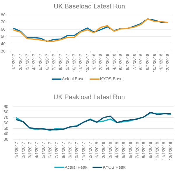
Figure 1: Monthly baseload power prices in a backtest of the KYOS fundamental market model. The graphs compare the average historical spot prices (‘Actual’) with the backcast values from the model. Source: Charles River Associates Inc.
Forecast power prices and comparison to the market
Once the model has been validated on historical data, it is time for a price forecast. Figure 2 shows annual forecasts of for 6 European power markets, with a gradually rising trend, especially after 2025. The fuel forward prices, determining the costs of conventional generation, are taken from settlement prices on the 14th of April 2020 and extrapolated by 2% annually after 2025. The carbon prices are from the same trading date, and extrapolated a bit more aggressively by 5% annually after 2027.
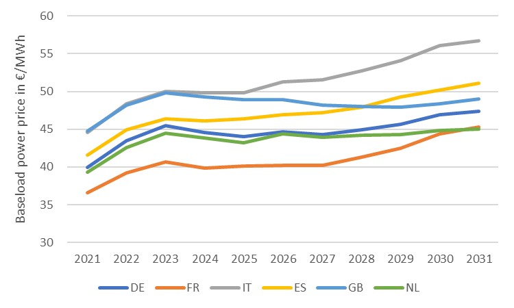
Figure 2: Annual baseload power price forecasts for 6 European markets. The forecasts are generated with the KYOS fundamental power market model KyPF. Source: KYOS.
Among the many fundamental modelling assumptions between this and other figures are a small increase in electricity consumption and a strong rise in the solar and wind capacities. These increases are projected on the actual demand, solar production, and wind production in 2018, as if the future weather conditions follow the 2018 weather conditions exactly. In this context, 2018 is the so-called base year for the residual load forecast, making the results more realistic than with a smoothed residual load forecast. In order to generalize the results, the model can be run with multiple base years, for example 2016 and 2017.
Figure 3 contains the German power forecasts derived from the different base years, their average, and the EEX settlement prices from the 14th of April 2020. First of all, the differences between the base years are rather small, always well below 1 €/MWh. Secondly, the EEX settlement prices are below the fundamental forecast by 2 €/MWh on average in 2021-2023, and above the fundamental forecast by 1.3 €/MWh in 2024-2026. A potential explanation for the first three years is that the Covid-19 effect was not taken into account in the fundamental model, whereas the market might have priced in the effects of a demand slump, especially in 2021.
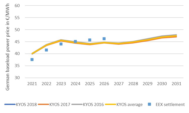
Figure 3: Annual baseload power price forecasts for Germany, using base years 2016-2018, compared to the settlement prices of baseload calendar forwards on EEX on 14th of April 2020. Source: KYOS / EEX.
Understanding the future supply stack
Over the years, there will be changes in the conventional generation park. Some of these changes can directly be derived from government plans and commercial investment and de-investment announcements. For example, according to law, nuclear capacities are to be phased out in Germany by 2023 and in Belgium by 2025. In Germany this coincides with a gradual reduction of the coal and lignite plants to a level of zero around 2035-2040. Because the net demand is not expected to decrease due to electrification in e.g. transport and the industry, and because solar and wind are not (much) available in many hours, the maximum required capacity remains roughly the same.
Consequently, the system would have black-outs in certain periods if this decrease in flexible generation assets were not compensated for by an increase in energy storage (see graph label: “pump hydro” in Figure 4) and gas-fired plants (graph label: “TTF”). So, most of the assumed increase in gas-fired generation and energy storage is an assumption which follows from the prerequisite that society will not accept black-outs. Some of these new capacities will earn enough money in the day-ahead power markets, others cannot do without the income from ancillary services to balance the system, while in some cases even capacity fees might be needed for a sound economic business case.
The generation mix will certainly undergo significant changes. This is what we see in figure 4, comparing the forecast production in January 2021 with January 2031. In both years, the residual demand peaks at about 60-65 GW. The lowest levels of residual demand are much lower in 2031 though, going below -10 GW. This summarizes the challenge for the future: average residual demand goes down, while the fluctuations become much larger. Gas-fired plants (in blue) and other conventional generation have a much peakier output profile in 2031 than in 2021. Furthermore, pump hydro and other forms of energy storage essential to maintain the system balance.
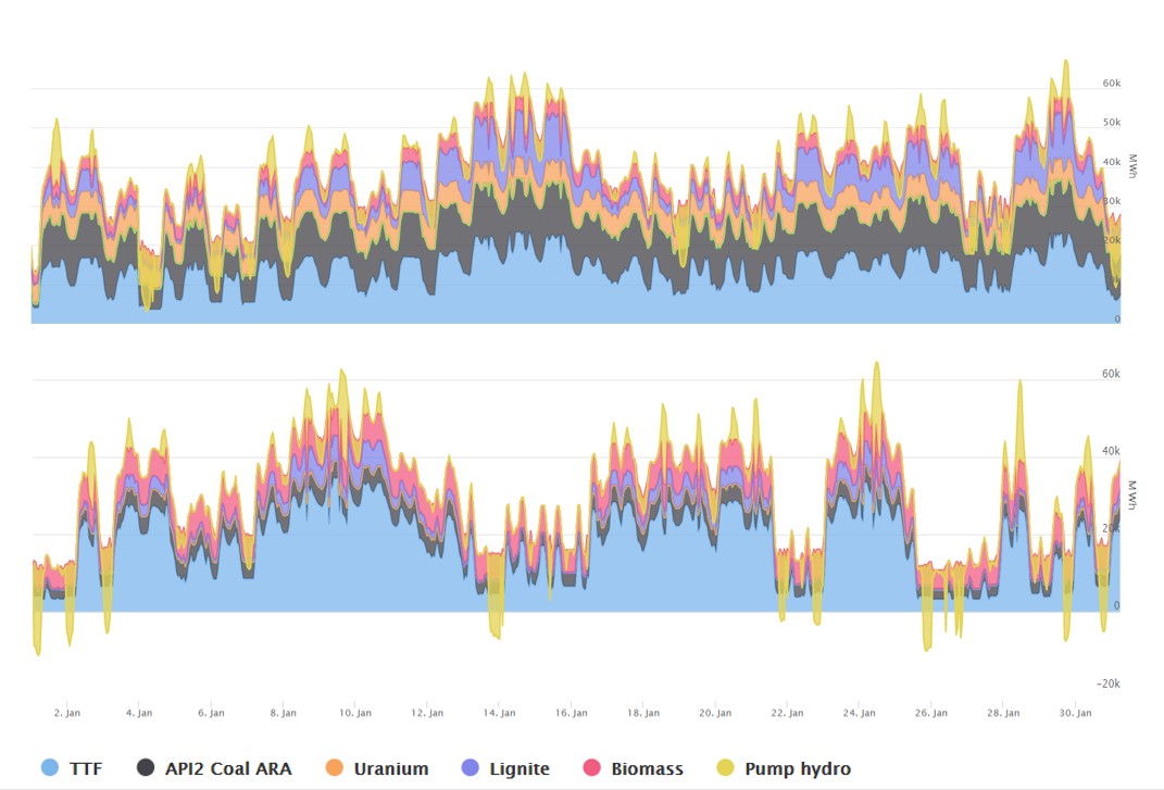
Figure 4: Forecast production from flexible generation in Germany in January 2021 (top) and January 2031 (bottom). The total production in each hour is equal to the German load minus the solar and wind production and minus the net import. TTF is the generation from gas, API2 Coal ARA from steam coal, Uranium from nuclear, Lignite from lignite, Biomass from biomass or biogas, and Pump hydro from pump hydro facilities, batteries and other forms of energy storage. Note that the last category also has negative production, during hours of energy storage. Source: KYOS KyPF model.
VALCOE, not LCOE
It has become standard practice to compare the economics of renewable power technologies by their Levelized Cost of Energy (LCOE). The LCOE equals the fixed and variable costs over the lifetime of the asset, divided by the number of production hours. However, this concept does not take into account the level of the power price in the hours of production. It also ignores the flexibility that some assets have to provide balancing services (most noticeable category: batteries) and it ignores the cannibalization effect.
An improved concept introduced by the IEA is the value-adjusted LCOE, or VALCOE [1] . For intermittent sources, it adds the cannibalization effect and balancing costs to the variable costs. Likewise, for flexible sources, it reduces the costs by the expected income from ancillary services. The net result is a fairer economic comparison between technologies providing flexibility (energy storage, most conventional assets) and requiring flexibility (most renewable assets).
Forecasting future capture rates
The VALCOE highlights the importance of the capture rate in the economics of a renewable asset. As explained earlier, the capture rate is the average realized spot price for the renewable asset divided by the equally weighted (baseload) average spot price.
Capture Rate=(Average Realized Spot Price)/(Average Baseload Spot Price)
So far, capture rates have been fairly close to 100%. With increasing levels of renewables penetration, capture rates are likely to be pushed down. For example, in its “Renewable Cannibalisation Problem”[2] report, ICIS forecasts Spanish solar capture rates to fall to about 50% in 2030. Their baseload power price forecast is around 44, while the average realized spot price for solar is forecasted at just 22 €/MWh.
The KYOS fundamental power market model can forecast capture rates for any country and any type of technology. The only prerequisite is to have a full year of hourly historical weather data for the renewable asset, so either wind speed data or solar radiation. This allows the model to include the output of the renewable asset in the supply stack of the market, and calculate the average realized spot price.
This is displayed in figure 5 for the two assets that were introduced in article 4: the Dutch North-Sea wind farm and the solar PV park in the middle of Spain. The figure shows a drop of the Spanish solar capture rate from currently around 99% to 88% in 2030 and 79% in 2036. For the Dutch wind output, the drop is not so steep and ends in 2036 at 89%. Although not as extreme as the ICIS forecast, the discounts to the baseload prices are economically significant nonetheless, especially in 2036: almost 11 €/MWh for the Spanish solar and almost 6 €/MWh for the Dutch off-shore wind. Such discounts have important implications for the value of long term PPAs and the negotiated terms.
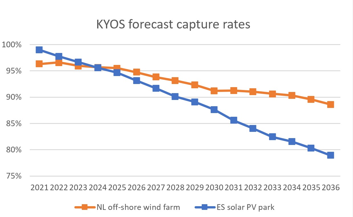
Figure 5: Forecast capture rates for two renewable assets: a Dutch off-shore wind farm and a Spanish solar park. Source: KYOS KyPF model.
Prices and capture rates
This was the third and last article about creating long-term price forecasts. For long-term forecasts, beyond around five years, a fundamental model is an indispensable tool. It allows users to generate a price forecast for the market baseload price, but also for the expected realized price of specific assets. Of course, many assumptions have to be made, for example about the level of fuel prices and the speed by which the whole energy transition takes place. It means in practice you will be running several scenarios and calculate sensitivities to deepen your understanding of your asset or PPA and be well prepared for any price negotiation.
Feedback on our “Financials of renewable Power and PPAs”
We write the articles to share our knowledge and hope it provides a useful source of information for newcomers and experienced professionals alike. Each article will be a mix of qualitative description, some mathematical formulations and numerical examples. Whether you are buying electricity for your company, developing new projects, working for a utility, providing financing, drafting policies, or just generally interested: we hope you read the articles with interest and share your feedback with us: info@kyos.com.
To view this article in pdf: Valuing long-term investments and PPA contracts – the financials of renewable power and PPA contracts
[1] https://www.iea.org/reports/world-energy-model/techno-economic-inputs
[2] https://sdgresources.relx.com/sites/default/files/renewable-cannibalisation-white-paper.pdf